Have I missed any important Twitter communities?

I searched Twitter for 24 hashtags, and it is entirely possible that I have missed a few important ones. By looking at the most frequent hashtags in the corpus I should be able to see if I have missed anything important.

To start, I need to import all of the tweets from their CSV files.

library(tidyverse)
file_names <- list.files("~/data/twitter", full.names = TRUE)
tweet_files <- vector(mode = "list", length = length(file_names))
for (i in seq_along(file_names)) {
  tweet_files[[i]] <- read_csv(file_names[i])
}
tweets_raw <- bind_rows(tweet_files)
tweets_raw %>% select(fullname, text)

## # A tibble: 411,153 x 2
##    fullname        text                                                   
##    <chr>           <chr>                                                  
##  1 𝓟𝓪𝓸𝓵𝓸           Differential expression analysis with Bioconductor and…
##  2 Paul Blaser     Gene Ontology analysis with #Python and #Bioconductor …
##  3 Lalit Kapoor    #bioconductor for analyzing genome data.. hmm looks in…
##  4 Darren Wilkins… Looking for a CDF (or a #bioconductor cdf package) for…
##  5 Davide          Nice #R and #bioconductor manual http://faculty.ucr.ed…
##  6 Seth Falcon     Pair programming some improvements to the graph packag…
##  7 Chris Lasher    Eff it, I'm going for a ride. I'll resume beating my h…
##  8 Neil Saunders   Error in dyn.load(file, DLLpath = DLLpath, ...) undefi…
##  9 Michael Dewar   is anyone an #Rstats #bioconductor genius? I have a ne…
## 10 Ricardo Vidal   Somewhat abusing biomaRt... #R #Bioconductor           
## # ... with 411,143 more rows

I also need to de-duplicate the dataset, as there are many tweets that used multiple hashtags and I don’t want to give them unnecessary weight.

tweets <- tweets_raw %>% select(-html) %>% distinct
pct_unique <- ( nrow(tweets) / nrow(tweets_raw) ) * 100
glue::glue("There are {nrow(tweets)} unique tweets out of \\
           {nrow(tweets_raw)} total ({round(pct_unique,2)}% unique).")

## There are 403833 unique tweets out of 411153 total (98.22% unique).

Using the tidytext package I can now do a little bit of text mining to see if there are any important hashtags I should add to my Twitter search list.

library(tidytext)
tweet_hashtags <- tweets %>% 
  unnest_tokens(word, text, "tweets", strip_punct=TRUE) %>% 
  filter(str_detect(word, "^#")) %>% 
  count(word, sort = TRUE)
tweet_hashtags

## # A tibble: 61,704 x 2
##    word                  n
##    <chr>             <int>
##  1 #rstats          377405
##  2 #datascience      57521
##  3 #bigdata          18830
##  4 #python           16435
##  5 #machinelearning  13993
##  6 #dataviz          11703
##  7 #analytics        10479
##  8 #r                10179
##  9 #ai                6905
## 10 #r4ds              6315
## # ... with 61,694 more rows

Nothing is jumping out as me (I’m looking for hashtags which are indicative of a community that I might have missed) so I think I’ll stick with my current list of hashtags.

Can I plot this using ggraph?

I’ve got a niggling feeling that I’m going to encounter problems with the scale of the dataset. igraph is written in C so it should scale fairly well, but with over 400,000 tweets it is important to get a feel for how these packages are going to perform on my laptop. If I can calculate the graph from my previous post (which was built from only 1,500 tweets) then I’ll be a lot more comfortable with my ability to do the rest of the project using igraph (and tidygraph/ggraph by extension).

library(rtweet)
library(igraph)
library(ggraph)

rt_g <- tweets %>% 
  filter(retweets > 0) %>% 
  select(user, text) %>% 
  unnest_tokens(word, text, "tweets", strip_punct=TRUE) %>% 
  filter(str_detect(word, "^@")) %>% 
  mutate(word = str_remove(word, "@")) %>% 
  graph_from_data_frame()

V(rt_g)$node_label <- unname(ifelse(degree(rt_g)[V(rt_g)] > 20, names(V(rt_g)), "")) 
V(rt_g)$node_size <- unname(ifelse(degree(rt_g)[V(rt_g)] > 20, degree(rt_g), 0)) 

ggraph(rt_g, layout = 'linear', circular = TRUE) + 
  geom_edge_arc(edge_width=0.125, aes(alpha=..index..)) +
  geom_node_label(aes(label=node_label, size=node_size),
                  label.size=0, fill="#ffffff66", segment.colour="slateblue",
                  color="red", repel=TRUE, fontface="bold") +
  coord_fixed() +
  scale_size_area(trans="sqrt") +
  labs(title="Retweet Relationships", subtitle="Most retweeted screen names labeled. Darkers edges == more retweets. Node size == larger degree") +
  theme_graph() +
  theme(legend.position="none")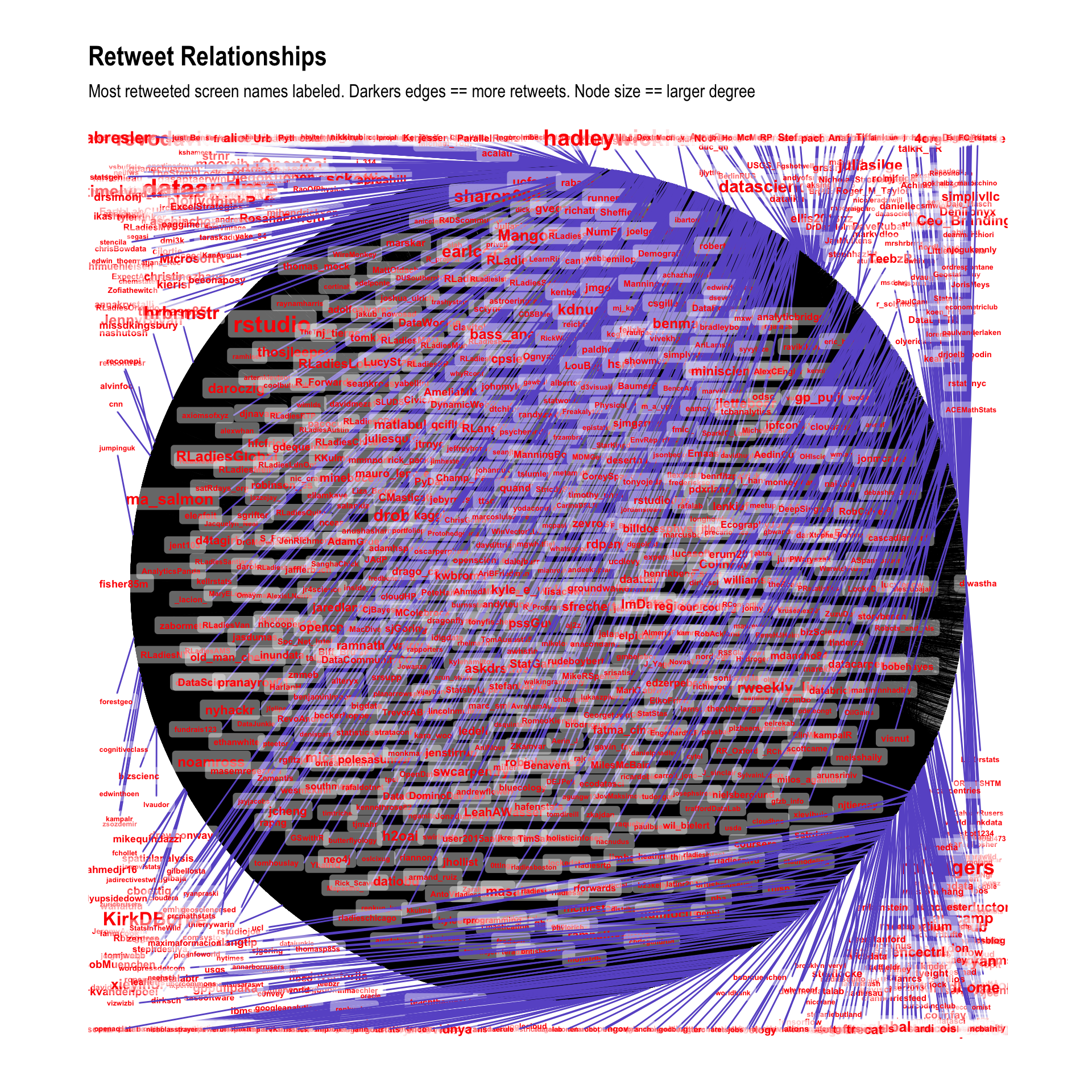

Well that looks terrible, but the point of this activity is showing that igraph/tidygraph/ggraph will work with this much data. It took a fair while to finish calculating, but it got there in the end. For now I will call this a success as it looks like I should be able to work on this project without any special tools.

I’m happy with both the data and the tooling, so I think I’m ready to start on the analysis now!