Setting up OAuth

If you’re running something like this for the first time, you will need to register your application with Twitter and authenticate with OAuth. You only need to do this process once - as long as you have a valid token (and you have the location of that token stored in the TWITTER_PAT environment variable) then you don’t need to do this every time you want to connect to Twitter.

twitter_token <- create_token(
  app = Sys.getenv("TWITTER_APP"),
  consumer_key = Sys.getenv("TWITTER_CONSUMER_KEY"),
  consumer_secret = Sys.getenv("TWITTER_CONSUMER_SECRET")
)
saveRDS(twitter_token, "~/.rtweet.rds")

Now we can test that everying is working by grabbing the top Twitter trends for Sydney.

aus_trends <- get_trends("sydney")
aus_trends %>% select(trend)

## # A tibble: 42 x 1
##    trend                  
##  * <chr>                  
##  1 #UFC229                
##  2 Quentin Kenihan        
##  3 Andrew Gaff            
##  4 #ConstellationCup      
##  5 Safety Car             
##  6 #repTourDallas         
##  7 #BTSxCitiField         
##  8 Argentina              
##  9 #Banksy                
## 10 Productivity Commission
## # ... with 32 more rows

These sure don’t match the trends for Sydney on the Twitter website, which is almost exclusively sporting hashtags at the moment. Thankfully we don’t really need to figure out what’s broken here as we won’t be using Twitter’s trends functionality, but at least we can confirm that the OAuth token is working.

Grabbing some #rstats tweets

If everything does what it says on the box, then I should be able to grab a big pile of tweets with just one command: rtweet::search_tweets(). Let’s give it a go!

rstats_sample <- search_tweets("#rstats", n = 1000, include_rts = FALSE)
rstats_sample %>% select(name, text) %>% sample_n(10)

## # A tibble: 10 x 2
##    name               text                                                
##    <chr>              <chr>                                               
##  1 uwe sterr          "I just😍  knitr::include_url, use it in #bookdown a…
##  2 Agnese Vardanega   A very very simple function to export tables in csv…
##  3 Thomas Hütter      Posted by Alex Joseph, now on R-bloggers: Comparing…
##  4 R-bloggers         Three new domain-specific (embedded) languages with…
##  5 Bio Lab Analytics… Principal components analysis (PCA) is a powerful #…
##  6 Emily Webb         #rstats https://t.co/twi1YZQpQC                     
##  7 LIBD rstats club   "We are getting closer to publishing our blog post …
##  8 R-bloggers         America – get ready for EARL! https://t.co/zl4cRtoL…
##  9 Tyler Morgan-Wall  Don't worry, I didn't forget about 3D ggplot render…
## 10 R-bloggers         12 Best Data Science Resources on the Internet http…

We can now have a bit of a dig into the data to see who has been getting lots of retweets, and what they have been tweeting about.

top_retweets <- rstats_sample %>% 
  group_by(name) %>% 
  tally(retweet_count, sort=TRUE)
top_retweets

## # A tibble: 469 x 2
##    name                     n
##    <chr>                <int>
##  1 Dr. GP Pulipaka        925
##  2 R-bloggers             712
##  3 Kirk Borne             359
##  4 Mine CetinkayaRundel   254
##  5 Mara Averick           184
##  6 RStudio                155
##  7 Aspioneer              131
##  8 Hank Hershey            58
##  9 Sharon Machlis          55
## 10 boB Rudis               33
## # ... with 459 more rows

rstats_sample %>% 
  arrange(desc(retweet_count)) %>% 
  select(retweet_count, name, text)

## # A tibble: 983 x 3
##    retweet_count name           text                                      
##            <int> <chr>          <chr>                                     
##  1           254 Mine Cetinkay… Teaching (with) R? Consider adding your c…
##  2           155 RStudio        r2d3: R Interface to D3 Visualizations ht…
##  3           152 Kirk Borne     Colossal Collection of Convenient Cheat S…
##  4            57 Hank Hershey   Coming soon to a github repository near y…
##  5            52 Sharon Machlis "My #rstats book Practical R for Mass Com…
##  6            47 Kirk Borne     Build a strong foundational knowledge of …
##  7            46 Kirk Borne     "A Big List of Lists of #DataScience and …
##  8            38 Kirk Borne     Chart Suggestions — a thought-starter for…
##  9            37 R-bloggers     Animating a Monte Carlo Simulation https:…
## 10            37 Dr. GP Pulipa… "Free eBook: Data Science Algorithms in a…
## # ... with 973 more rows

It is of course entirely unsurprising to find that Mara Averick (@dataandme) features on this leaderboard.

Turning Twitter data into a graph

I’ll stick to following the Bob Rudis book again here, with future blog posts to look at doing this in a more targeted way. For now the objectives are to:

• join all the dots together so I know I have my local R environment playing nicely with rtweet and igraph
• make some pretty images so I can make sure blogdown is ready for future blog posts

rstats <- search_tweets("#rstats", n=1500)

rt_g <- filter(rstats, retweet_count > 0) %>% 
  select(screen_name, mentions_screen_name) %>%
  unnest(mentions_screen_name) %>% 
  filter(!is.na(mentions_screen_name)) %>% 
  graph_from_data_frame()

V(rt_g)$node_label <- unname(ifelse(degree(rt_g)[V(rt_g)] > 20, names(V(rt_g)), "")) 
V(rt_g)$node_size <- unname(ifelse(degree(rt_g)[V(rt_g)] > 20, degree(rt_g), 0)) 

ggraph(rt_g, layout = 'linear', circular = TRUE) + 
  geom_edge_arc(edge_width=0.125, aes(alpha=..index..)) +
  geom_node_label(aes(label=node_label, size=node_size),
                  label.size=0, fill="#ffffff66", segment.colour="slateblue",
                  color="red", repel=TRUE, fontface="bold") +
  coord_fixed() +
  scale_size_area(trans="sqrt") +
  labs(title="Retweet Relationships", subtitle="Most retweeted screen names labeled. Darkers edges == more retweets. Node size == larger degree") +
  theme_graph() +
  theme(legend.position="none")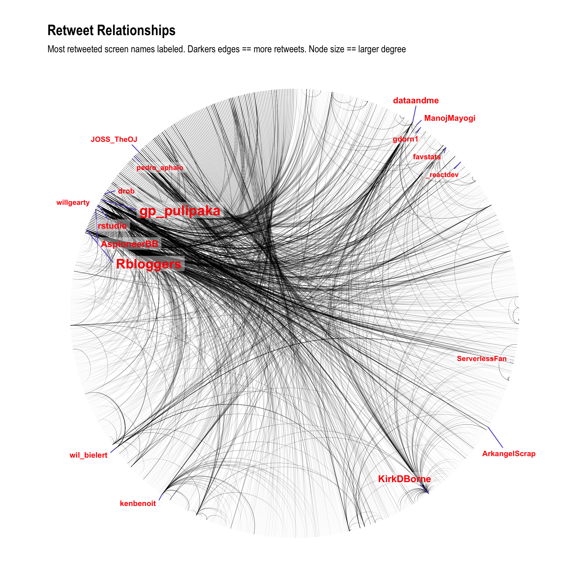

Cool! It worked!

For the next blog post I’ll look to take a much larger sample, cleaning up the mess that is “retweeting” (because retweets are important in the community, but producers are obviously more important) and then using the igraph to try and identify distinct communities.