Nodes and Edges

For this network the nodes will be hashtags, and the (undirected) edges will be co-occurrence of those hashtags in a single tweet. Node weights will be given by the total number of occurrences of the hashtag, and edge weights will be given by the number of occurrences of the pair of hashtags.

Firstly, I will load the data, extract the hashtage, and create the nodes:

library(tidyverse)
library(tidytext)

tweets <- readRDS("~/data/twitter-cache/tweets.rds")

hashtags <- tweets %>% 
  unnest_tokens(word, text, "tweets") %>% 
  filter(str_detect(word, "^#")) %>% 
  select("tweet-id", "word") %>% 
  rename(tweet = "tweet-id",
         name = "word")

hashtag_nodes <- hashtags %>% 
  count(name, sort = TRUE) %>% 
  rename(popularity = n)

That was easy, but the edges will be harder due to the structure of the data.

hashtag_edges <- hashtags %>% 
  
  # Use a join to generate all potential hashtag edges
  inner_join(hashtags, by = "tweet") %>% 
  rename(from = "name.x",
         to = "name.y") %>% 
  
  # Remove all edges which are going to/from the same node
  filter(from != to) %>% 
  
  # Exploit "a" < "b" = TRUE to remove one edge out of each bidirectional pair
  filter(from > to) %>% 
  
  # Tally the edge counts
  count(from, to, sort = TRUE)

That was easier than expected, thanks to the fact R let me test for alphabetical ordering using >. Hooray for operator overloading!

Creating the graph

This is really easy now, using the tidygraph package which in turn wraps around the igraph package.

library(igraph)
library(tidygraph)

# Using the igraph constructor as the tidygraph one is buggy
hashtag_graph <- hashtag_edges %>% 
  graph_from_data_frame(directed = FALSE, vertices = hashtag_nodes) %>% 
  as_tbl_graph()  

hashtag_graph

## # A tbl_graph: 61704 nodes and 273941 edges
## #
## # An undirected simple graph with 385 components
## #
## # Node Data: 61,704 x 2 (active)
##   name             popularity
##   <chr>                 <int>
## 1 #rstats              377405
## 2 #datascience          57521
## 3 #bigdata              18830
## 4 #python               16435
## 5 #machinelearning      13993
## 6 #dataviz              11703
## # ... with 6.17e+04 more rows
## #
## # Edge Data: 273,941 x 3
##    from    to     n
##   <int> <int> <int>
## 1     1     2 57496
## 2     1     3 18959
## 3     1     4 16356
## # ... with 2.739e+05 more rows

And of course now I’m going to try plotting it straight away with minimal cleaning!

library(ggraph)
library(particles)

hashtag_graph %>% 
  activate(nodes) %>% 
  top_n(30) %>% 
  ggraph() + 
  geom_node_point(aes(size = popularity)) +
  geom_node_label(aes(label=name, size=popularity),
                  label.size=0, fill="#ffffff66", segment.colour="slateblue",
                  color="red", repel=TRUE, fontface="bold") +
  geom_edge_arc(edge_width=0.25, curvature = 0.1, aes(alpha=n)) +
  theme_graph() +
  theme(legend.position="none")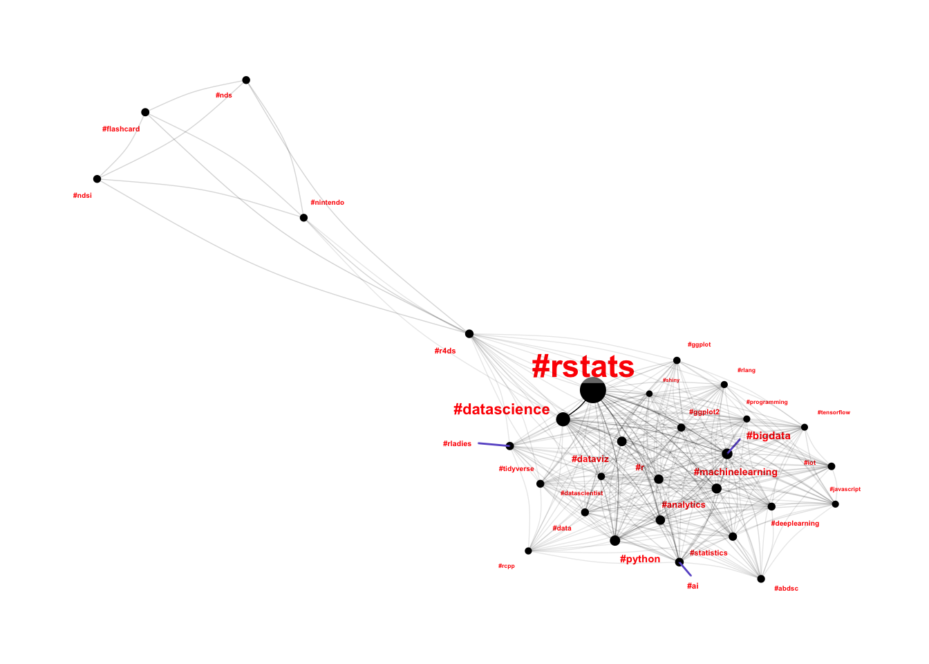

Consider me surprised 😮😮😮

Let’s take a look at these three seriously disconnected hashtags and see whether we have discovered a new community, or whether we’ve identified a hashtag clash on the #r4ds hashtag.

tweets %>% 
  filter(str_detect(text, "#nds")) %>% 
  select(text)

## # A tibble: 4,290 x 1
##    text                                                                    
##    <chr>                                                                   
##  1 NEW REVIEW : R4 SDHC Revolution Flashcard - http://bit.ly/7av2Z #r4 #SD…
##  2 R4i SDHC V1.4 Adaptor with Kingston TF 4G For Nintendo DSi 33.85$ http:…
##  3 R4 SDHC with Kingston MicroSD 2GB Memory Card 20.95$ http://bit.ly/iwfV…
##  4 DSTTi For Nintendo DSi 17.85$ http://bit.ly/m28JCl  #nintendo #flashcar…
##  5 R4DS SDHC with Kingston Micro SDHC 4GB Memory Card 24.95$ http://bit.ly…
##  6 R4i-SDHC V1.4.1 with Kingston TF 2GB Card 29.85$ http://bit.ly/lCZ7SU  …
##  7 R4i Ultra DSi Card with Kingston MicroSDHC 4GB Memory Card 31.52$ http:…
##  8 "M3i Zero Sakura   Kingston Micro SDHC 4GB Card \t40.95$ http://bit.ly/…
##  9 R4 SDHC with Kingston MicroSD 2GB Memory Card 20.95$ http://bit.ly/iwfV…
## 10 DSTTi For Nintendo DSi 17.85$ http://bit.ly/m28JCl  #nintendo #flashcar…
## # ... with 4,280 more rows

There is definitely a clash on #r4ds - it looks like someone called “R4” is selling #flashcards for the #nintendo DS… Let’s filter out tweets containing #nintendo and do this all again.

hashtags <- tweets %>% 
  filter(!str_detect(text, "nintendo")) %>% 
  unnest_tokens(word, text, "tweets") %>% 
  filter(str_detect(word, "^#")) %>% 
  select("tweet-id", "word") %>% 
  rename(tweet = "tweet-id",
         name = "word")

hashtag_nodes <- hashtags %>% 
  count(name, sort = TRUE) %>% 
  rename(popularity = n)

hashtag_edges <- hashtags %>% 
  inner_join(hashtags, by = "tweet") %>% 
  rename(from = "name.x",
         to = "name.y") %>% 
  filter(from != to) %>% 
  filter(from > to) %>% 
  count(from, to, sort = TRUE)

hashtag_graph <- hashtag_edges %>% 
  graph_from_data_frame(directed = FALSE, vertices = hashtag_nodes) %>% 
  as_tbl_graph()  

hashtag_graph %>% 
  activate(nodes) %>% 
  top_n(30) %>% 
  ggraph() + 
  geom_node_point(aes(size = popularity)) +
  geom_node_label(aes(label=name, size=popularity),
                  label.size=0, fill="#ffffff66", segment.colour="slateblue",
                  color="red", repel=TRUE, fontface="bold") +
  geom_edge_arc(edge_width=0.25, curvature = 0.1, aes(alpha=n)) +
  theme_graph() +
  theme(legend.position="none")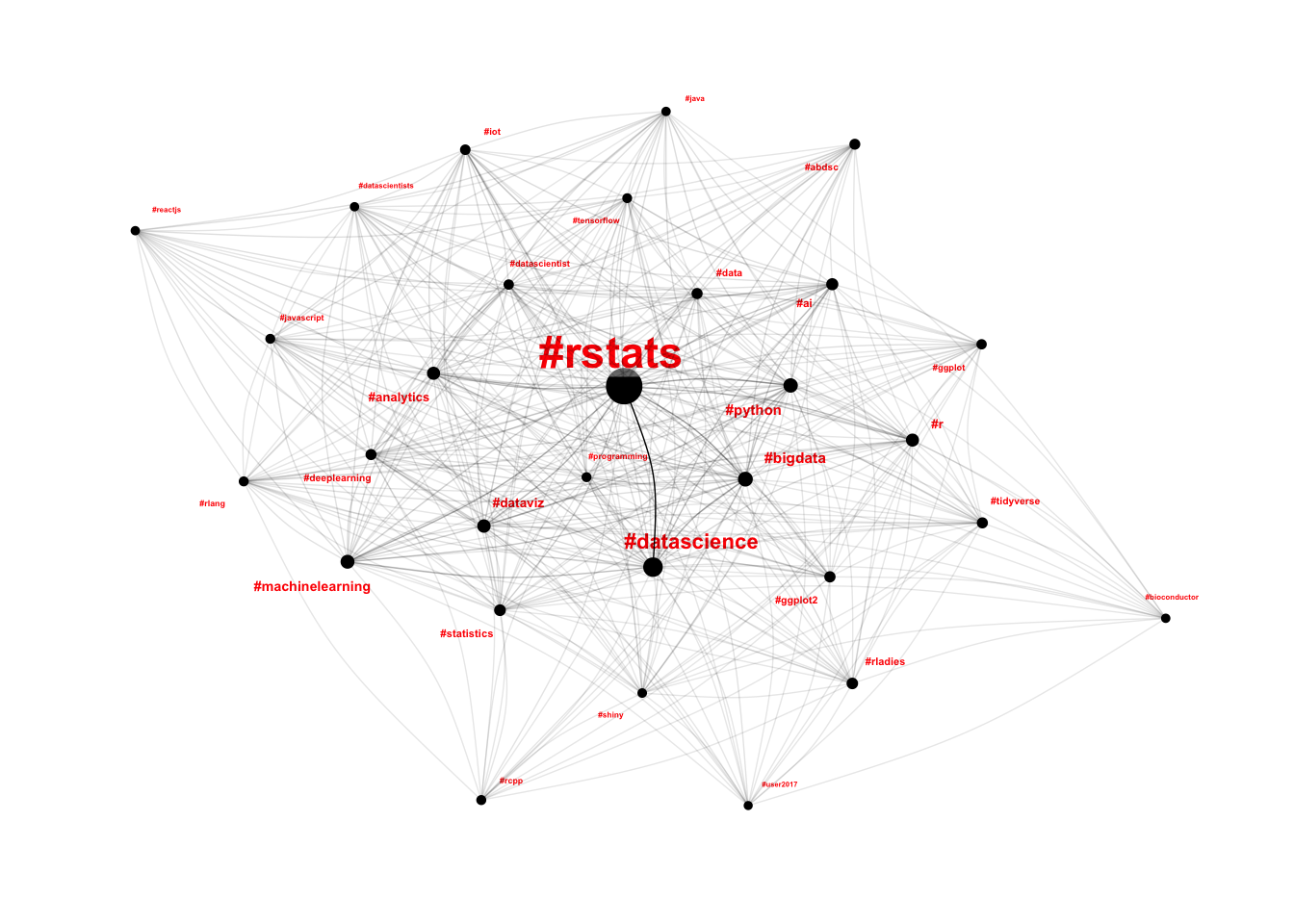

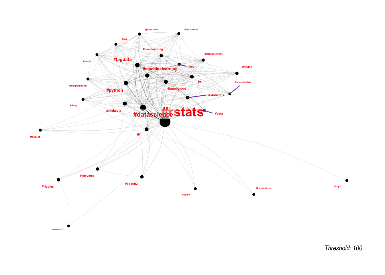
This is looking a little bit more like the hairball I expected. The layout is effectively random, and there aren’t really any clusters to exploit. This is mostly due to the fact that each edge has exactly the same importance as every other edge; if one tweet mentions #rcpp and #reactjs, then that edge is just as important as the edge representing the 57,496 tweets which mentioned #rstats and #datascience.

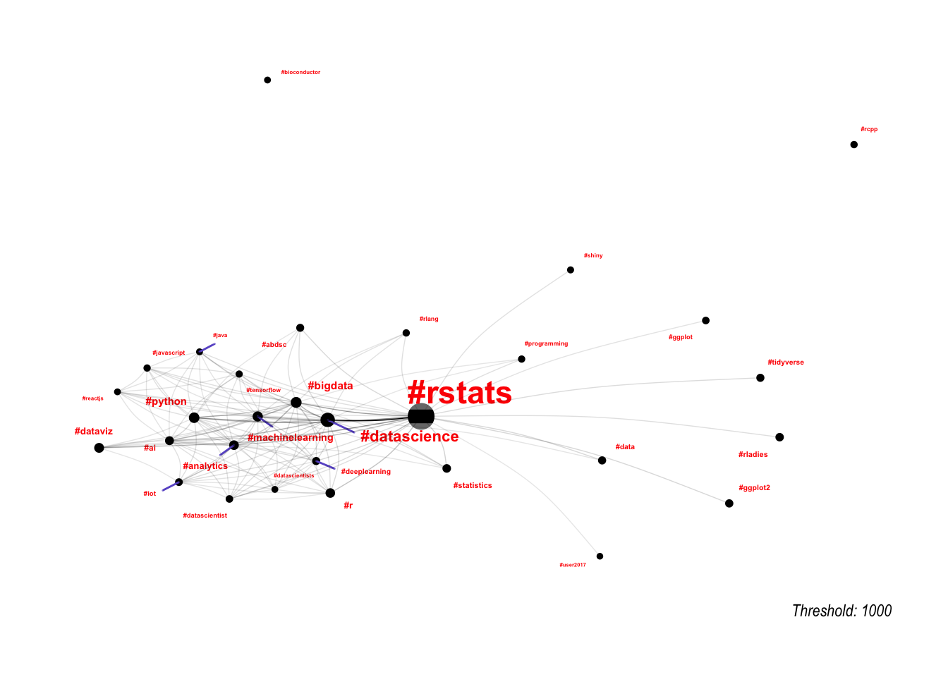
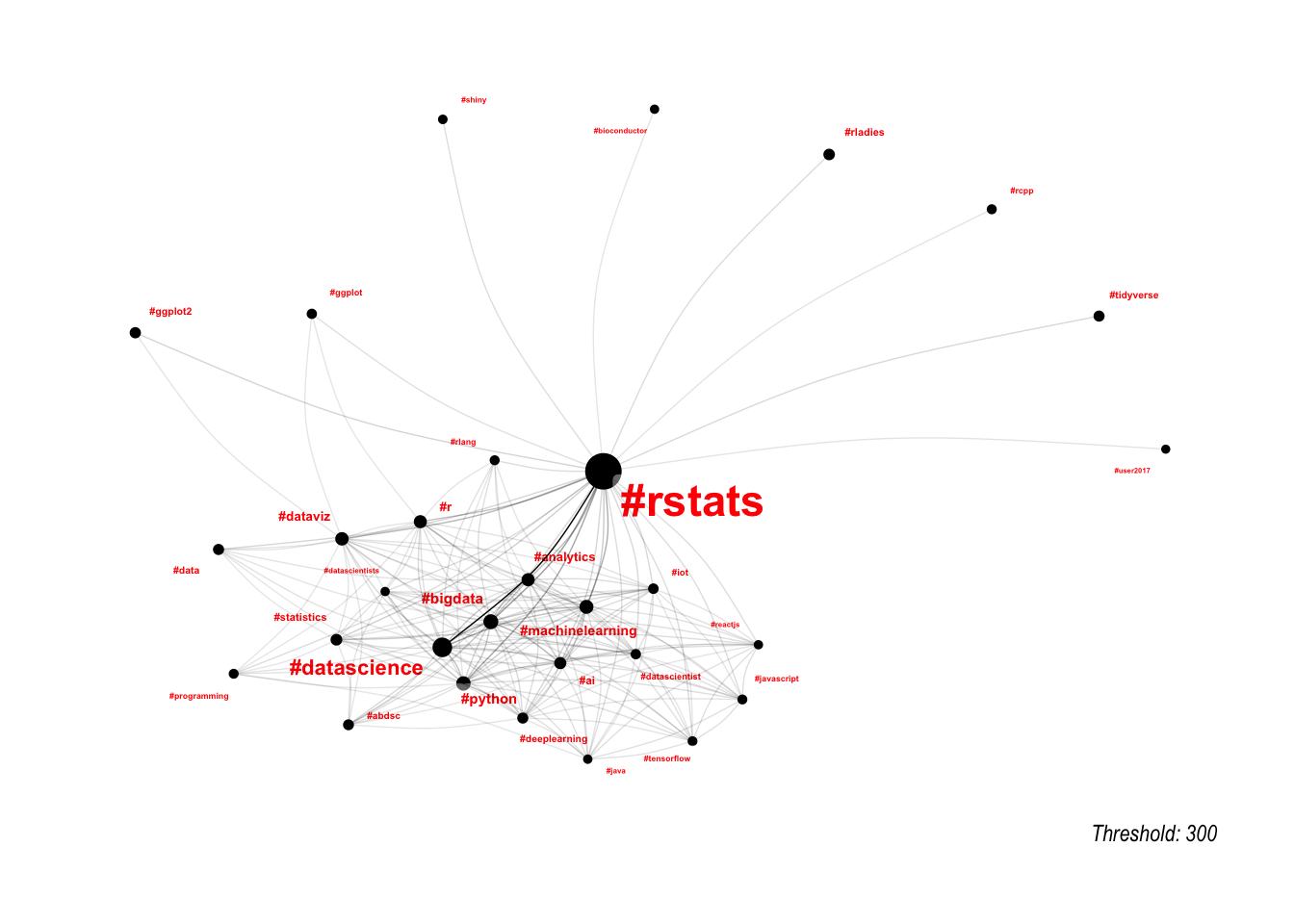
One way to deal with this is to set a threshold for edges, so that we only plot the most important edges. This works a little bit, but is very sensitive around the threshold selected.

lapply(c(1000, 300, 100), function(threshold) {
  hashtag_graph %>% 
    activate(nodes) %>% 
    top_n(30) %>% 
    activate(edges) %>% 
    filter(n >= threshold) %>% 
    ggraph() + 
    geom_node_point(aes(size = popularity)) +
    geom_node_label(aes(label=name, size=popularity),
                    label.size=0, fill="#ffffff66", segment.colour="slateblue",
                    color="red", repel=TRUE, fontface="bold") +
    geom_edge_arc(edge_width=0.25, curvature = 0.1, aes(alpha=n)) +
    theme_graph() +
    theme(legend.position="none") +
    labs(caption = paste0("Threshold: ", threshold))
})

A more generalisable method for taking these differences in edge importance into account is to use a force-directed graph, which we can do using the particles package.

library(particles)

hashtag_graph %>% 
  activate(nodes) %>% 
  top_n(50) %>% 
  simulate() %>% 
  wield(link_force, strength = n/max(n)) %>% 
  wield(manybody_force, strength = -30 * popularity/max(popularity)) %>% 
  wield(center_force) %>% 
  evolve() %>% 
  as_tbl_graph() %>% 
  ggraph(layout = "nicely") + 
  geom_node_point(aes(size = popularity)) +
  geom_node_label(aes(label=name, size=popularity),
                  label.size=0, fill="#ffffff66", segment.colour="slateblue",
                  color="red", repel=TRUE, fontface="bold") +
  geom_edge_arc(edge_width=0.25, curvature = 0.1, aes(alpha=n)) +
  theme_graph() +
  theme(legend.position="none")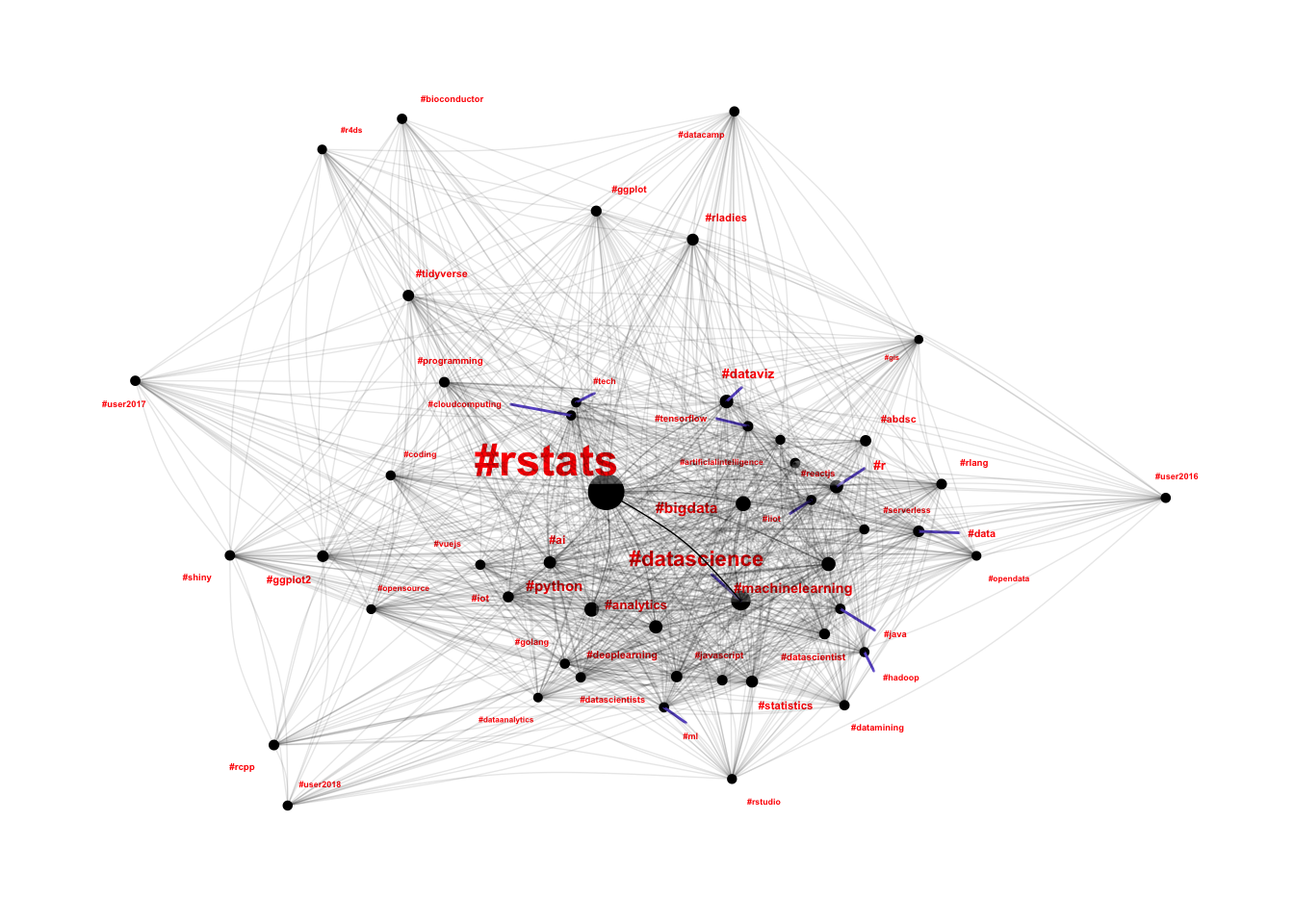

This is a little more like what I was expecting. Hashtags like #rcpp, #shiny, #bioconductor and even the UseR conference hashtags are well separated from the hairball. Known “strong” communities like #rladies and #r4ds are appearing towards the edges, and #rstudio (an occasionally polarising topic in the community) are also well outside the hairball. At first glance it is very interesting to see #rstats and #python so closely connected, however there is significant selection bias at play here as I have only scraped R tweets for this analysis, rather than bringing in all of the Python communities as well.

Community Detection

This isn’t likely to work very well I’m effectively looking for “communities of communities”. I have to limit the number of nodes for the community detection (as it is quite slow), which also doesn’t help the results.

hashtag_graph %>% 
  activate(nodes) %>% 
  top_n(500) %>% 
  mutate(community = as.factor(group_infomap(weights = n))) %>% 
  # top_n is broken because min_rank is broken, so I'm doing it from scratch
  filter(rank(desc(popularity), ties.method = "min") <= 50) %>% 
  simulate() %>% 
  wield(link_force, strength = n/max(n)) %>% 
  wield(manybody_force, strength = -30 * popularity/max(popularity)) %>% 
  wield(center_force) %>% 
  evolve() %>% 
  as_tbl_graph() %>% 
  ggraph(layout = "nicely") + 
  geom_node_point(aes(size = popularity)) +
  geom_node_label(aes(label=name, size=popularity, col = community),
                  label.size=0, fill="#ffffff66", segment.colour="slateblue",
                  repel=TRUE, fontface="bold") +
  geom_edge_arc(edge_width=0.25, curvature = 0.1, aes(alpha=n)) +
  theme_graph() +
  theme(legend.position="none")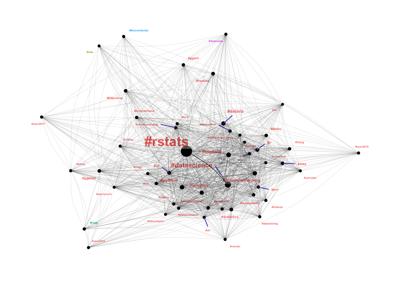

Well I guess that is a win - it detected some of the outlying communities! According to the algorithm #r4ds, #bioconductor, #datacamp and #rcpp are separate communities to the core #rstats community. I’ll dig into this further in a future post when I start plotting individuals rather than hashtags.

Final Notes

Overall I’m surprised at how powerful ggraph is, once you get the hang of it. The documentation for tidygraph is still quite sparse, and the package is a little buggy which cost me an hour or so of stuffing around. I’m generally thrilled with how easy it is to work with graphs using these packages, and I’m happy that the Twitter dataset is giving me something interesting to work with!